Source: https://www.maketecheasier.com/create-dr…8Make+Tech+Easier%29
Capture Date: 16.09.2018 22:41:30
Creating a dropdown list in your Excel spreadsheet can help to increase the efficiency of your work. This might come in handy, especially when you want your coworkers to provide certain information that may be relevant to the company. By using an Excel dropdown list, you can control exactly what can be entered into a cell by giving the users an option to select from a pre-defined list.
When you add a dropdown list to a cell, an arrow will be displayed next to it. Clicking on this arrow will open up the list and give the user the option to choose one of the items on the list. This will not only save you space on your spreadsheet but also make you look like like a superuser and impress your co-workers and boss. Here’s a step-by-step guide on how to create a dropdown list in Excel.
Step 1: Define the Contents of Your List
1. Open up a new Excel worksheet and put down the contents you want to appear on your list. Make sure each entry occupies one cell, and all entries are vertically aligned in the same column. Also, ensure there are no blank cells between the entries. In our case our dropdown menu will open a list of cities to choose from.

2. Once you’re done assembling the list, highlight all the entries, right-click on them, and select “Define Name” from the menu that will show up.

3. This will open a new window with the title “New Name.” Choose a name for your list and enter the same in the “Name” text box.

4. Click “OK.”
Step 2: Adding Your Dropdown List to a Spreadsheet
The next step is to add your dropdown list to a spreadsheet. Here’s how to do it.
1. Open a new or existing worksheet where you want to place your dropdown list.
2. Highlight the cell where you want to place the dropdown list. Click the “Data” tab, then locate the “Data validation” icon in the data tools section and click on it.

3. A data validation box will appear that has three tabs: Settings, Input Message, and Error Alert. In the Settings tab, select “List” from the “Arrow” dropdown list. A new option titled “Source” will now appear at the bottom of the window. Click the text box and then enter a “=” sign, followed by the name of your dropdown list. In our case it should read =cities.
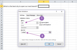
The “Ignore blank” and “In-cell dropdown” boxes are checked by default. With the Ignore blank cell checked, it means it’s okay for people to leave the cell empty. But if you want every user to select an option from the cell, uncheck the box.
4. Click OK. That’s it. You have added a dropdown list to your spreadsheet.

With that completed, you can now proceed to the Input message tab.
Step 3: Set Input Message for Data Validation (Optional)
At times you may want a message (with description) to pop up when the cell containing the dropdown list is clicked. In that case you’ll need to click the “show input message” box in the Input message tab. You’ll also need to fill out the title and the input message in their respective boxes. Your dropdown list should now look something like the following image.
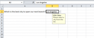
The last tab is for the error alert. Once defined, this one sends an error message if someone enters invalid data – data that is not on the list.
Wrapping Up
Dropdown lists are very common on websites and are very intuitive for the user. Their versatile nature renders them useful in virtually all industries. Be it in surveys, the business world or even in schools, you’ll always find the need to use Excel dropdown lists.
Was this article useful? Feel free to comment and share.